
Phishing Websites Capstone Project
The following is a mock problem I posed for myself to contextualize my findings.
Full Code Repo
Data and Dictionary Repo
Problem statement
With the ever-expanding reach of digital technology, online security savviness of the average internet user must expand, too. For this reason, a web browser company has asked its data science team to predict whether a website is “phishing” for information from vulnerable users. The company aims to use the findings from the team’s report to display a redirect message to its users indicating that they are clicking on a link that may potentially steal their information.
Data
Data overview
Data: UCI Machine Learning (ML) Archive
Each of the datasets number rows contains an observation of one website as well as its phishing status, determined by an expert. Some 30 features of the dataset include “Redirect”, “Favicon”, and “URL_length”, each of which will be further explained in the report. The dataset is provided by the web browser company, and all variables collected were predetermined to be of at least some interest in deciding whether a website is a phishing website or not.
Loading the data
I loaded the data as a Pandas dataframe called ‘data’ into my Python environment from a ‘.csv’ file. I had several flat file options in addition to ‘.csv’ such as ‘.arff’ and ‘.xslx’, but ‘.csv’ proved to be the most convenient. The data consisted of 31 column names in the first row, and values in the following 11055 rows. The data did not contain any additional information such as comments, extra sheets, definitions, etc., which is why I did not specify any additional arguments when loading the data.
Resetting the index to start at 0.
The original raw data had an ‘index’ column that started with the integer 1. The reason I didn’t load the ‘index’ column available in the data as a Pandas index is because I wanted my index column to start at 0 to match the Python convention. I did this through a series of column transformations.
Renaming the columns to be more legible
The raw data had column names with repeating words (e.g. ‘URLURL_Length’ and ‘having_IPhaving_IP_Address’), misspelled words (e.g. ‘Shortining_Service’), and not consistently capitalized words (e.g. ‘having_At_Symbol’). I renamed the columns to be more legible and more easily understandable, by making each column name lowercase, separating each word with an underscore, and changing some names to better match the meaning of the values (e.g. ‘Domain_registeration_length’ to ‘domain_registeration_period’).
Data dictionary
Due to the nature of the data provided by the original source: M. Mohammad, Thabtah, and McCluskey, the values available in the data were not clear. All features were optimized for machine learning through a conversion to 2 or 3 categorical values such as ‘-1,1’ or ‘-1,0,1’. Fortunately, a column definition document was provided by the original owners of the data and is available in the GitHub project folder. Unfortunately, the document doesn’t clearly specify which human-understandable values map onto which values in the dataset. This is where I had to make informed decisions to map the values.
My methodology consisted of a combination of prior knowledge, relying on the data document, and looking at the ‘result’ variable to match the values available in the data to the definitions in the data document. I then put this information into a nested dictionary for easy graphing, information extraction, and analysis in the future. The other option was to make a copy of the data and replace every value with a human-understandable definition, but for space complexity reasons, I chose to go with a hash table instead.
Missing values & outliers
I first checked each column for null values using the Pandas ‘.isnull()’ method. This returned no missing values. I then ran a ‘set’ function over every column of the data frame to check for non-traditional or misspelled missing values such as ‘N/A’, ‘NUL’, ‘na’, ‘missing’, etc. The results of this function confirmed the results above, meaning no unexpected entries existed in any of the columns.
Traditional methods for checking for outliers such as boxplots, histograms, and scatterplots were not applicable with the raw data, because every variable was categorical. So, using the set method discussed above, I also check for outliers, which resulted in no visible outliers. In the next steps of this project, where I take a look at the data visually, outliers that were not found with the ‘set’ method, might show up then.
Exploratory Data Analysis - Overview
To get a good idea of what the data look like, I made a composite stacked bar graph showing the label variable distribution for each feature. Below is an example of one feature that I explain in detail in a later paragraph.
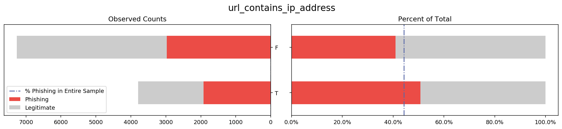
On the left is a stacked bar graph of the total counts of phishing vs legitimate websites within each of the two categories of the feature ‘url_contains_ip_address’, namely ‘T’ and ‘F’. This bar shows how the counts of ‘T’ and ‘F’ compare to each other, as well as how the distribution of phishing vs legitimate websites looks for each category.
On the right is a stacked bar that shows the proportion of legitimate websites for each of the categories of the feature shown. By changing the x-axis from counts to percentage I hope to make it easy to see the difference in proportions of phishing websites for each category ‘T’ and ‘F’. I also add a reference line representing what proportion phishing websites make up of the original data in order to show not only how the categories compare to each other but also to the sample average.
I repeated this process for every feature in the dataset, resulting in 30 plots available in the code of this project. After generating these plots I looked through them to see which features stray the furthest away from the sample average. These will likely be the features that my models will use in the future to predict the label, which gives me direction for some statistical inference.
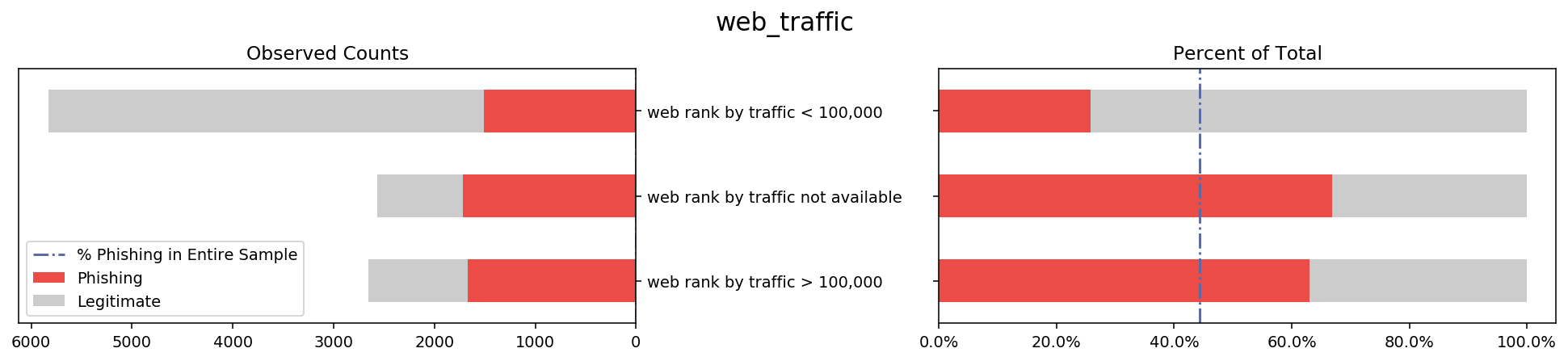
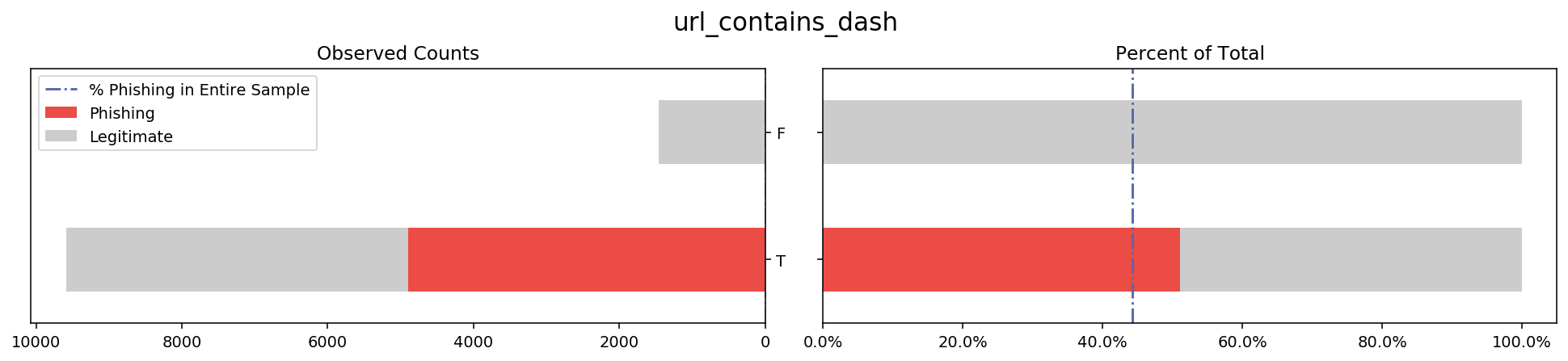
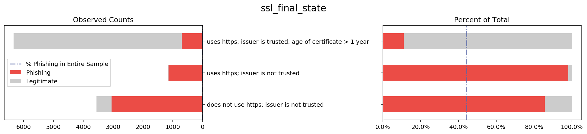
Below I listed several other graphs where the bars tend to stray away from the overall sample proportion because these variables might have a lot of decision power in the prediction stage. While these visualizations served to get me familiar with the data, in a later stage I will apply more rigorous methods that will allow me to make stronger claims about which columns are important.
pal = ['#eb4c46', '#cccccc'] #choice of colors

# overall sample proportion of phishing websites
prop_phish = pd.DataFrame((data.groupby('result').size())/(data.groupby('result').size().sum())).loc[-1, 0]

# for loop that prints the viz for each feature
for column in data.columns:
    if column == 'result':
        pass
    else:
        # Figure specs
        fig = plt.figure(figsize=(14, 3), dpi=140)
        fig.suptitle(column, fontsize=16, y=1.05)

        # Divide the figure into a 1x2 grid, and give me the first section
        ax1 = fig.add_subplot(121)

        # Divide the figure into a 1x2 grid, and give me the second section
        ax2 = fig.add_subplot(122)

        # Left groupby and plot
        g_count = data.groupby([column, 'result']).size().unstack('result') # count of each category
        g_count.plot.barh(stacked = True, ax = ax1, color = pal).invert_xaxis() # barplot
        ax1.yaxis.tick_right()
        ax1.set_ylabel('')
        ax1.set_yticklabels(data_dict[column].values())
        ax1.axvline(0, color='#5868a8', linewidth=1.5, linestyle = '-.', label = 'Horizontal') # adding only for the legend (not visible line)
        ax1.legend(labels=['% Phishing in Entire Sample', 'Phishing', 'Legitimate'])
        ax1.set_title('Observed Counts')


        # Right groupby and plot
        g_count2 = data.groupby([column, 'result']).size().unstack(column)
        p = g_count2.divide(g_count2.sum())
        plot2 = p.transpose().plot.barh(stacked = True, ax = ax2, color = pal)
        ax2.get_legend().remove()
        ax2.axvline(prop_phish, color='#5868a8', linewidth=1.5, linestyle = '-.')
        ticks = np.round(ax2.get_xticks()*100)
        ax2.set_xticklabels(['{:}%'.format(j) for j in [str(i) for i in ticks]])
        ax2.set_ylabel('')
        ax2.set_yticklabels('')
        ax2.set_title('Percent of Total')

        fig.tight_layout()

Statistical Inference
The barplot visualization shows that some features stray further from the sample proportion of phishing websites than others. To develop some hypotheses about what features will be influential in model selection, I first filtered down to the ‘interesting’ features with the following method. For each category of each feature, I ran a 10,000 size bootstrap sample of the ‘result’ label variable. I then took this information to calculate a 99.9% confidence interval for the proportion that phishing websites made up of that group. If the overall proportion of phishing websites in the whole sample was outside of the 99.9% CI for at least two of the categories of a feature, I labeled that feature as ‘interesting’. The number of phishing websites that have these ‘interesting’ features will either be significantly higher or lower than the sample average, at 99.9% confidence. This might then suggest that these features will have a lot of influence when building models and may have high predictive power in whether a website is phishing or legitimate. Below is a list of the ‘interesting’ columns.
# Defining necessary functions to see which groups are interesting
def one_minus_mean(data):
    result = 1 - np.mean(data)
    return result


# courtesy of https://campus.datacamp.com/courses/statistical-thinking-in-python-part-2/bootstrap-confidence-intervals?ex=6
def bootstrap_replicate_1d(data, func):
    return func(np.random.choice(data, size=len(data)))

def draw_bs_reps(data, func, size=1):
    """Draw bootstrap replicates."""

    # Initialize array of replicates: bs_replicates
    bs_replicates = np.empty(size)

    # Generate replicates
    for i in range(size):
        bs_replicates[i] = bootstrap_replicate_1d(data, func)

    return bs_replicates

# changing this to be able to take mean of the bootstrap samples.
data.result[data.result == -1] = 0


# big checking function
# bootstrap replicates
# function automatically selects columns where the pop. prop. of phishing is outside the CI

high_interesting_columns = []
low_interesting_columns = []

for i in data.columns[:30]:    # excluding the result variable
    for j in set(data[i]):     # iterating over possible cateogies
        loop_data = data.result[data[i] == j]    # getting result variable for each category of each feature
        bs_replicates = draw_bs_reps(data=loop_data, func=one_minus_mean, size=10000)
        ci = np.percentile(bs_replicates, [.05, 99.95])
        if ((prop_phish < ci[0])): #interested in the high proportions
            high_interesting_columns.append(i)
        elif ((prop_phish > ci[1])): #low interesting columns
            low_interesting_columns.append(i)

    if high_interesting_columns != []:    # check for error when list is empty
        if sum(np.array(high_interesting_columns) == i) == 1:    # removing any columns where only 1 feature was out of CI
            high_interesting_columns.remove(i)
    if low_interesting_columns != []:    # check for error when list is empty
        if sum(np.array(low_interesting_columns) == i) == 1:    # removing any columns where only 1 feature was out of CI
            low_interesting_columns.remove(i)

high_interesting_columns = list(set(high_interesting_columns))    # removing duplicate entries
low_interesting_columns = list(set(low_interesting_columns))

print('Interesting columns with CI above sample proportion:', high_interesting_columns)
print('Interesting columns with CI below sample proportion:', low_interesting_columns)
Interesting columns with CI above sample proportion:
[‘ssl_final_state’, ‘web_traffic’, ‘url_contains_sub_domain’]
Interesting columns with CI below sample proportion:
[‘links_pointing_to_page’, ‘url_of_anchor’, ‘sfh’, ‘links_in_tags’]
Merely looking at a list of feature names doesn’t tell me too much, so the next step would be to visualize the features somehow.
Exploratory Data Analysis - Closer Look
To visualize the data within the ‘interesting’ columns, I want to display the proportion of phishing websites within each combination of categories for each combination of features. Below is a crosstab example of what I mean, as well as the relevant code.
| sfh | -1 | 0 | 1 |
|---|---|---|---|
| links_pointing_to_page | |||
| -1 | 0.62 | 0.56 | 0.79 |
| 0 | 0.46 | 0.64 | 0.80 |
| 1 | 0.54 | 0.69 | 0.77 |
# Creating a hash table of every combination of interesting columns
# Each key in hash table contains heatmap table of combinations of interesting columns

# custom aggregation function
def prop(series):
    return round(sum(series)/len(series), 2)

#scalable solution
def heatmap_dict(heatmap_dict, interesting_columns):
    heatmap_dict = {}

    for i in range(len(interesting_columns)):
        for j in range(i+1, len(interesting_columns)):
            working_df = data[[interesting_columns[i], interesting_columns[j], 'result']].\
                         groupby([interesting_columns[i], interesting_columns[j]]).agg(prop).unstack(interesting_columns[j])

            working_df.columns = working_df.columns.droplevel() # remove 'result' from columns multindex

            heatmap_dict[interesting_columns[i], interesting_columns[j]] = working_df

    return heatmap_dict

# Running the above function on both 'high' and 'low' interesting columns
low_heatmap_dict = {}
low_heatmap_dict = heatmap_dict(low_heatmap_dict, low_interesting_columns)
high_heatmap_dict = {}
high_heatmap_dict = heatmap_dict(high_heatmap_dict, high_interesting_columns)
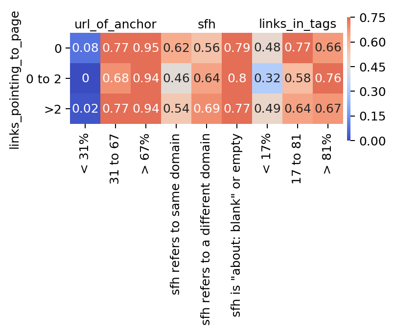
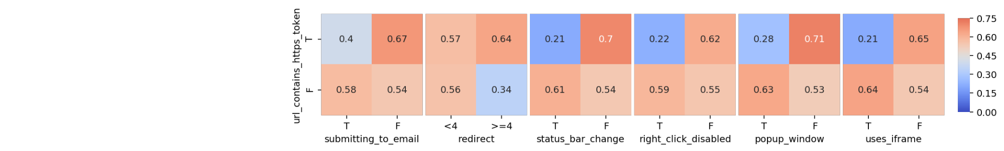
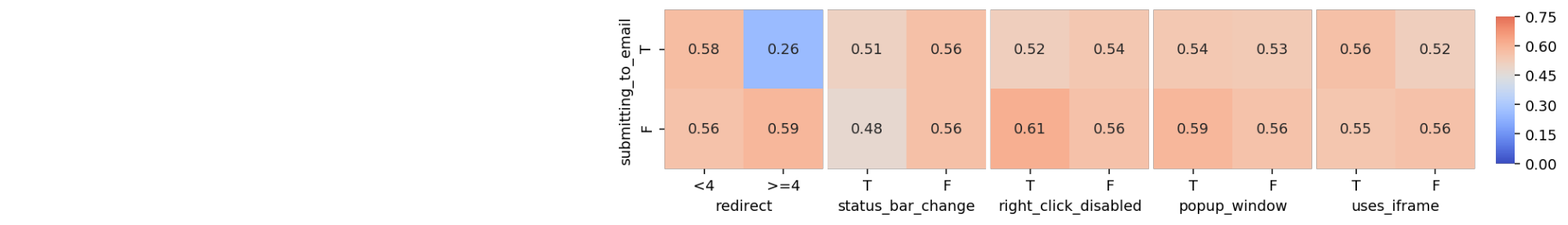
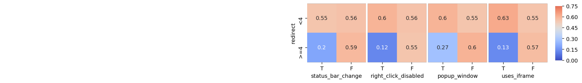
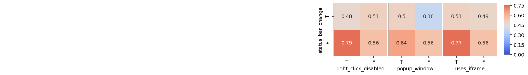
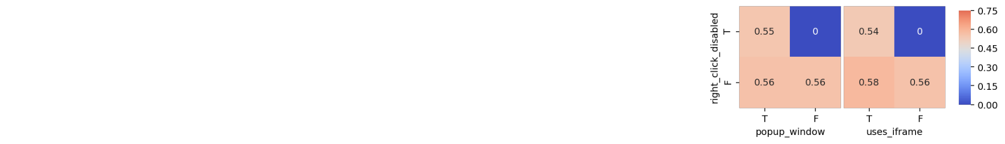
In this crosstab, each combination of each category is plotted and the number it contains inside is the proportion of phishing websites of that group. Notice that this crosstab only compares two features: ‘sfh’ to ‘links_pointing_to_page’, whereas in my full analysis I want to compare each combination of features, and visually display the proportions of phishing websites, as shown below. The color switches from shades of blue to shades of red, depending on whether the proportion of phishing websites for each specific combination in the visualization is above or below the sample proportion of phishing websites. The darker the color, the bigger the absolute difference between the combination proportion and the sample proportion.
# Scalable plotting function of the above plots

def prop_phish_heatmap(heatmap_dict, interesting_columns):
    for i in range(len(interesting_columns)-1):    #number of rows of entire heatmap

        fig, axes = plt.subplots(nrows=1, ncols=len(interesting_columns)-1, figsize=(4,2), dpi = 180)    # num of columns with particular size
        plt.subplots_adjust(wspace=0, hspace=0)    # space between subplots
        cbar_ax = fig.add_axes([.91, .15, .01, .7])    # location of color bar

        for j, (k, ax) in zip(range(i+1, len(interesting_columns)), enumerate(axes)):

            im = sns.heatmap(heatmap_dict[interesting_columns[i], interesting_columns[j]], ax = axes[k+i], #puts blanks in beginning
                        square=True, annot = True, cmap='coolwarm', center=prop_phish,
                        yticklabels = list(data_dict[interesting_columns[i]].values()),    #legible labels
                        xticklabels = list(data_dict[interesting_columns[j]].values()),
                        cbar=k == 0, cbar_ax=None if k else cbar_ax, vmin = 0, vmax = 0.75) #colorbar details
            ax.xaxis.set_label_position('top')

            if ax in axes[1:9]:
                axes[k+i].set_ylabel('')
                axes[k+i].set_yticklabels('')
                axes[k+i].tick_params(axis='y', length=0)
                # only keeps the y label for the first plot in each row

        for l in range(0,i):
                axes[l].axis('off')
                # I got it to work.
                # removes all labels from blank plots

#Plotting
prop_phish_heatmap(high_heatmap_dict, high_interesting_columns)
prop_phish_heatmap(low_heatmap_dict, low_interesting_columns)
It’s interesting to note some patterns that emerge. For example, despite the number of links_pointing_to_page, the url_of_anchor has a clear pattern showing the websites with a small url_of_anchor portion tend to not be fishing websites. Another example is just how important sfh seems to be when the website contains an ‘about:blank’ section. From other heatmaps available in the Python Notebook, there are also some unexpected surprises in terms of trends, but most confirm what the bar graphs showed.
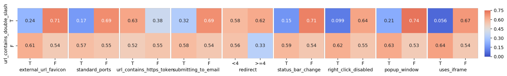
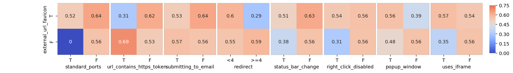
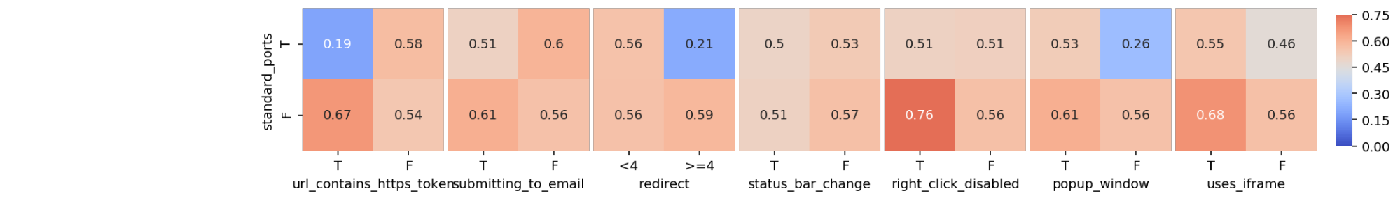
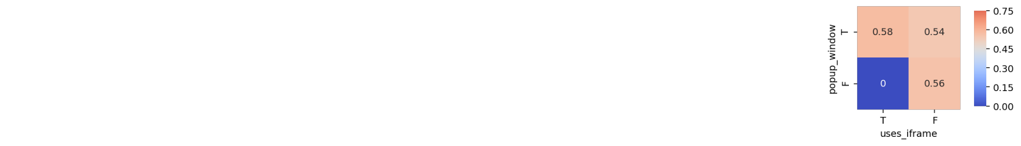
To show the scalability of this visualization method, I graphed all the non-interesting columns against each other to look for patterns that might be surprising. It’s interesting to note that there are several combinations that are made up of only legitimate websites.
Despite the versatility of this method, the machine learning portion of this report will be a far better measure of important columns along with the results of the model.
Machine Learning and Results
I tried the following ML models: untuned and tuned Logistic Regression, untuned and tuned Random Forest (RF), and untuned and tuned XGBoost models. I also used a combination of GridSearchCV and RandomizedSearchCV to tune the models. Each step provided me with a better fitting model, the procedure and results of which I discuss below. Additionally, I compare the models to each other at the end of this section.
Initial Considerations
Because the data is entirely categorical, there is no collinearity between the features to worry about. Also for this same reason, there are no greatly varied scales from variable to variable, and as I will show in the following section, the two label categories are balanced. My assumption for this project is that this dataset is randomly picked, or in another way representative of the population of interest.
Initial Train/Test Split
I created a train/test split for the data with a test size of 30%, meaning I used 70% of my data to train and tune my models with Cross-Validation (CV) splits and held 30% of the data untouched to then give a final test of the model. I used a stratified train/test split to make sure that both the train and test splits had the same proportion of phishing websites. The result was that 55.699% of the train set was phishing and 55.683% of the test set was phishing - a close enough result for my purposes.
Models
Logistic Regression
To tune the C parameter, one of the main hyperparameters to tune in logistic regression, which is defined as “Inverse of regularization strength” on the scikit website, I set up a sequence of numbers in the following logspace np.logspace(-10, 10, 100). On the scikit learn website, the definition of logspace is as follows: “the sequence starts at base^start (base to the power of start) and ends with base^stop”, with the specified amount of elements in the sequence. For my purposes, I set up a sequence that starts at 10^(-10), and ends at 10^(10), with 100 equally spaced numbers. This sequence gave me a lot of options to try out and zoom in on the best for my data.
I then did a comprehensive GridSearch with 5 CV folds of the parameter sequence and found the optimal C value of 0.7925. To make sure I picked the proper C value, I ran a RandomizedSearchCV of the same sequence as above and plotted it against the score of the resulting model. Below is a figure showing this.
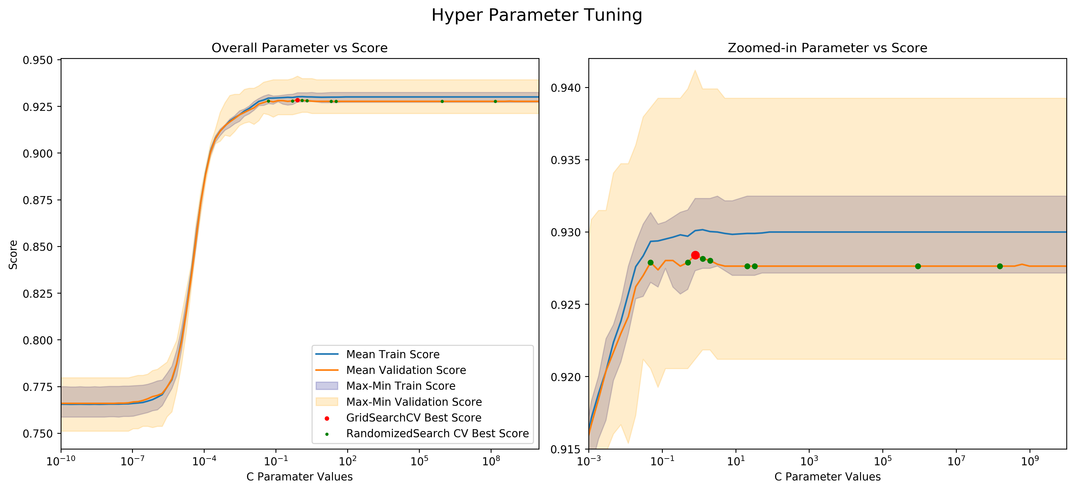
Across the logistic x-axis are the 100 possible values that C can take on. On the y-axis is the score of the resulting function. For each possible C value I got the train scores and validation scores through the validation_curve() function with 5 CV folds. This resulted in a score for each possible C value of the following:
- Validation data scores
- Min - lower value of orange band
- Mean - orange line
- Max - higher value of orange band
- Train data scores
- Min - lower value of blueband
- Mean - blueline
- Max - higher value of blue band
- Red dot - Optimal function picked through GridSearchCV
- Green dots - optimal functions picked by performing 10 RandomizedSearchCV
- Note there aren’t 10 dots, meaning some dots lie on top of each other
- Note there aren’t 10 dots, meaning some dots lie on top of each other
One interesting observation from the above graph is that even though RandomizedSearcCV doesn’t take as much computing power, it also might not produce consistent results because it doesn’t search the whole parameter grid. GridSearchCV, on the other hand, picks the optimal value but is more computationally expensive. Depending on the problem at hand, it might be useful to use RandomizedSearchCV (i.e. when quick “good enough” results are needed), or it might be useful to use GridSearchCV(i.e. when every last bit of model performance is necessary at the cost of computational effort).
Another interesting observation of the above graph is that the orange line along with its band is not fully below the blue line with its band. If this were the case, I would know that my model is overfitting as it is consistently underperforming on new data. Luckily, this is not the case for me. The validation band is broader than the train band, and the validation line is slightly below the train line. This is expected for two reasons: the variety and unknown nature of new data accounts for the wide band, and the new data being new accounts for the model’s drop in performance.
Logistic Regression Results
To compare Logistic Regression with other methods, the best Area Under the ROC Curve (AUC) that I got with Logistic regression was 0.9788 .
Random Forest Classifier
The next model I tried was the Random Forest (RF) Classifier. Now that I have introduced the general concepts of parameter tuning through GridSearch and RandomziedSearchCV, I won’t spend much time talking about them here. I built a parameter grid of the following parameters:
random_grid = {'n_estimators': n_estimators,
               'max_features': max_features,
               'max_depth': max_depth,
               'min_samples_split': min_samples_split,
               'min_samples_leaf': min_samples_leaf,
               'bootstrap': bootstrap}
For each parameter, I picked a variety of values, all of which are available in the Jupyter notebook for this project. Because of the large amount of possible parameters, I used RandomizedSearchCV to save some time but still come up with a usable result.
RF Classifier Results
After all the tuning, the best AUC score was 0.995 .
XGBoost
The final model I tried was the XGBoost model, a model with many parameters requiring the most tuning out of any model I tried. Because of the large amount of parameters, I tuned them one to three at a time, got the results and tuned the next batch of parameters. The final tuned model had the following parameters:
tuned_xgb = XGBClassifier(learning_rate =0.11, #tuned
                          n_estimators=2000,
                          max_depth=13, #tuned
                          min_child_weight=0, #tuned
                          gamma=0, #tuned
                          subsample=0.775, #tuned
                          colsample_bytree=0.9, #tuned
                          objective= 'binary:logistic',
                          nthread=4,
                          scale_pos_weight=1,
                          reg_alpha = 1e-05, #tuned
                          reg_lambda = 1, #tuned
                          seed=27)
XGBoost Results
The best XGBoost model, whose parameters are shown above produces an AUC score of 0.9969, the best so far.
Comparing All Models
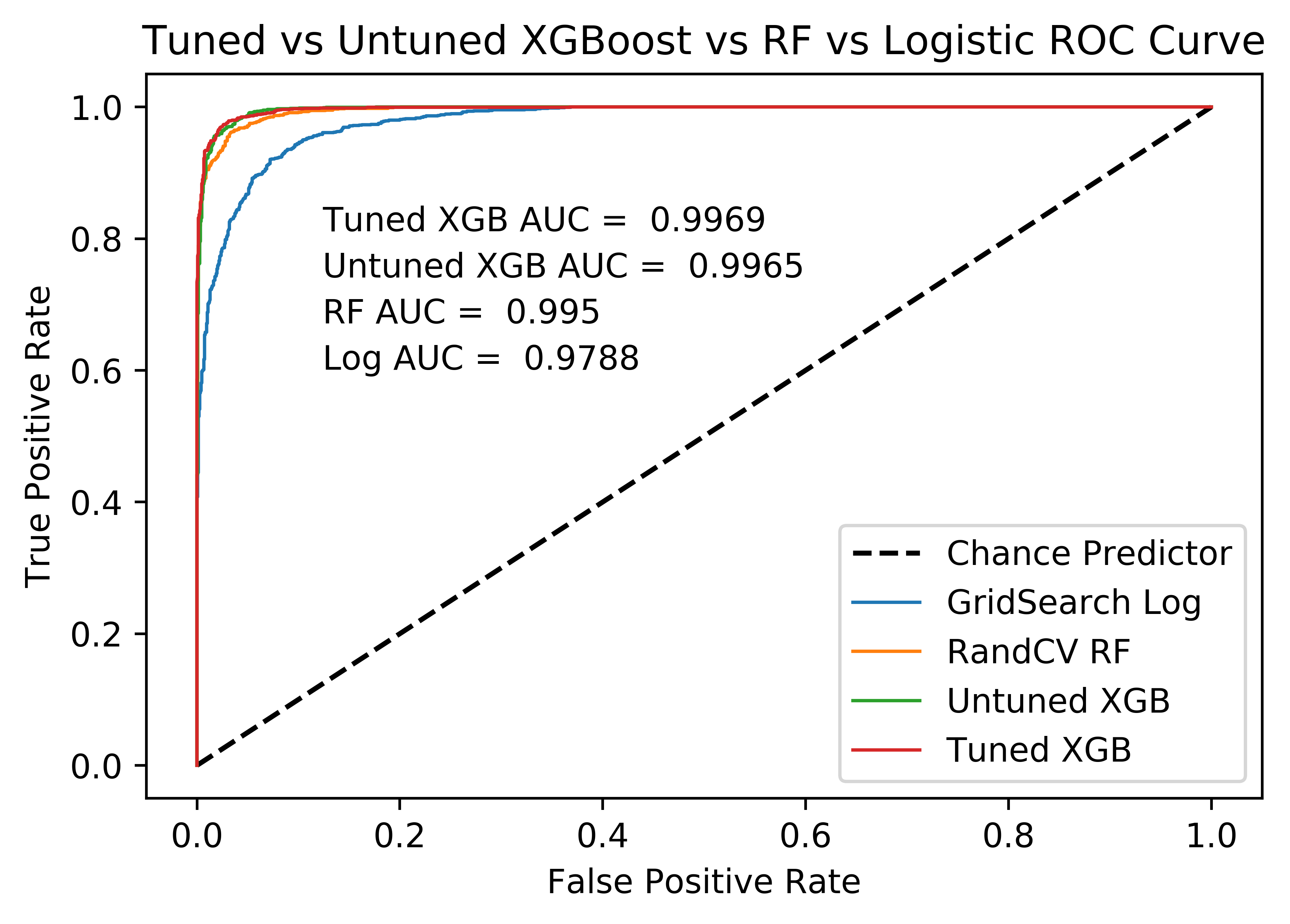
The figure above shows the ROC curves of all the models I tried in this section. The dotted line shows the ROC curve of a model that guesses randomly between the two categories: phishing and legitimate. Then in blue is the tuned Log Regression model, followed by the RF model, and the untuned and tuned XGBoost model. Note that even the untuned XGBoost model performed better than the tuned RF and tuned Logistic Regression models. This implies that at least for this classification problem, the XGBoost model is a great choice. Also note that the tuned XGBoost produced slightly better results than the untuned model, but the two ROC curves almost look identical. This seems to be an example of the widely known phenomenon of the law of diminishing marginal returns, in which with every additional unit of input, output becomes ever decreasingly favorable. In the case of tuning an already good model, this means that by putting in an additional hour of work into tuning the model, only slight positive changes will happen to the model’s performance.
Project Conclusion
In this project I explored, analyzed, and visualized the phishing website data in order to build a classifier that can tell whether a website is phishing or legitimate, as per the (mock) request of a large internet browser provider that wants to keep their users safe from malicious websites. After looking into the data and training several models, I delivered my best tuned XGBoost model as my final classifier to be deployed in real time to analyze websites and inform customers when they are about to enter a potentially phishing website.