
Real Estate Predictions part 2 - Kaggle
Introduction
In this project I take a dive into real estate data with the House Prices: Advanced Regression Techniques competition on Kaggle. This competition serves as a first step for beginners to “get their feet wet” with advanced regression and machine learning by predicting real estate prices based on a combination of qualitative and quantitative predictors.
As a machine learning novice, I thought this would be a great project to take on and learn more about linear regression, generalized linear modeling, random forests, parameter tuning, data imputation, and multicollinearity through R packages such as caret, XGBoost, mice, randomForest, and others.
Data Overview
In this project, I use the Real Estate Data, provided by Kaggle to up-and-coming data scientists looking for a real-world challenge, to analyze various quantitative and categorical predictors to predict housing prices. Similar processes are utilized by real estate companies to estimate the price of houses and inform their consumers about the value of a house based on factors such as its size, location, proximity to schools, etc.
Because of the vast differences between real estate markets in different parts of the world, the dataset for this project focuses on the market in Ames, Iowa. The data comes divided into a training set and a test set. The only difference between the two is that the training set contains the sale price and serves as the dataset that is used to train the model. Meanwhile, the test dataset doesn’t contain sale price, as that is the variable that is to be predicted.
There are 1,460 rows (observations) in the training dataset, representing individual houses at the point of sale. The dataset also features 81 columns (variables), 79 of which are explanatory, such as the size of the house, the condition of various aspects of the house (exterior, interior, basement, etc.), the neighborhood the house is in, number of rooms (bedrooms, bathrooms, etc.), and many others. The other two variables is an Id variable and the Sale Price variable, which is what we are predicting. Below is a list of all the variables in the dataset. Although many are self explanatory, a data dictionary is also available.
List of variables in the dataset
"Id"            "MSSubClass"    "MSZoning"      "LotFrontage"
"LotArea"       "Street"        "Alley"         "LotShape"
"LandContour"   "Utilities"     "LotConfig"     "LandSlope"
"Neighborhood"  "Condition1"    "Condition2"    "BldgType"
"HouseStyle"    "OverallQual"   "OverallCond"   "YearBuilt"
"YearRemodAdd"  "RoofStyle"     "RoofMatl"      "Exterior1st"
"Exterior2nd"   "MasVnrType"    "MasVnrArea"    "ExterQual"
"ExterCond"     "Foundation"    "BsmtQual"      "BsmtCond"
"BsmtExposure"  "BsmtFinType1"  "BsmtFinSF1"    "BsmtFinType2"
"BsmtFinSF2"    "BsmtUnfSF"     "TotalBsmtSF"   "Heating"
"HeatingQC"     "CentralAir"    "Electrical"    "X1stFlrSF"
"X2ndFlrSF"     "LowQualFinSF"  "GrLivArea"     "BsmtFullBath"
"BsmtHalfBath"  "FullBath"      "HalfBath"      "BedroomAbvGr"
"KitchenAbvGr"  "KitchenQual"   "TotRmsAbvGrd"  "Functional"
"Fireplaces"    "FireplaceQu"   "GarageType"    "GarageYrBlt"
"GarageFinish"  "GarageCars"    "GarageArea"    "GarageQual"
"GarageCond"    "PavedDrive"    "WoodDeckSF"    "OpenPorchSF"
"EnclosedPorch" "X3SsnPorch"    "ScreenPorch"   "PoolArea"
"PoolQC"        "Fence"         "MiscFeature"   "MiscVal"
"MoSold"        "YrSold"        "SaleType"      "SaleCondition"
"SalePrice"
There are 38,068 rows (observations) in the dataset, representing each college during 5 academic years 2012-2016, inclusive (e.g. Benedict College is featured 5 times, once for each year 2012- 16, inclusive). For year 2012, 7793 colleges were recorded; for year 2013, 7804 colleges were recorded; for year 2014, 7703 colleges were recorded; for year 2015, 7593 colleges are recorded; and for year 2016, 7175 colleges were recorded. The dataset also features 142 columns (variables) such as the name of the university, the location, various SAT/ACT score metrics, etc. that get populated with respective values about each college.
In the dataset, disregarding academic year, the 5 states with the most colleges are California with 3881 colleges, Texas with 2381 colleges, New York with 2317 colleges, Florida with 2176 colleges, and Pennsylvania with 2022 colleges. Similarly, disregarding academic year, the 5 states/territories with the fewest colleges are American Samoa with 5 colleges, Federated States of Micronesia with 5 colleges, Marshall Islands with 5 colleges, Northern Mariana Islands with 5 colleges, and Palau with 5 colleges. When I did this calculation by taking the average amount of colleges per year across the dataset, I got the same results. I also got the same results when I only looked at the most recent year.
I hypothesize that the top 5 states match the top 5 states by population, and similarly the bottom 5 states/territories match the bottom 5 states/territories by population. My hypothesis largely matches reality, with 4 out of 5 most populous states also being in the top 5 by college count (Pennsylvania is the exception). The least populated regions in the US are territories, so my hypothesis is supported as well.
Initial Data Wrangling
To set a baseline result, I wanted to run a simple linear regression using all the available predictors that contained at least 90% non-missing values. To do this, I changed all the text fields to factors and took out any columns that had over 90% missing values. Additionally, I did no imputation nor dummy variable assignment.
Initial Modeling
LM/GLM/GLMNet
Because of all the missing values, the lm() function could not predict all the rows, so for the rows that it couldn’t predict, I took the average value of all the other predictions and imputed the missing predictions with the average. I then did the same with glm() and glmnet() functions and compared the results.
The results are calculated as follows, and are shown below for the three methodologies discussed.
\[RMSE = \sqrt{\frac{1}{n}\Sigma_{i=1}^{n}{\Big({log(predicted_i) - log(actual_i)}\Big)^2}}\]| Results | |
|---|---|
| Function | RMSE |
| lm() | 0.47938 |
| glm() | 0.47581 |
| glmnet() | 0.47183 |
Secondary Data Wrangling
Now that a baseline was set, the real work could begin. I went through all the variables in the dataset and cross-referenced them with the data dictionary to see if the data dictionary could provide any insight into the nature of the data and more specifically, the missing values. Evidently, most of the missing values in the dataset were intentional and actually carried information. For a lot of the factor variables, a missing value meant the lack of a feature, as exemplified by variables such as BsmtQual, BsmtCond, FireplaceQu, and others, where an NA value means that the feature was missing.
Imputation
This discovery, however, doesn’t mean that some of the NA values were mistakes. For example, if BsmtQual was not missing, but BsmtCond was, then we know that that can’t be because they are related and if one is not missing, then the other must not be missing as well. In these cases, which were few and far between, I imputed the missing value with my best estimate for the specific house. For example, if I had to impute BsmtCond, I looked to other condition related variables for the house, such as overall condition, pool condition, conditions of various rooms, etc. Because there cases of missing factor variables were few and far between I found that manual imputation was the best way of dealing with these missing variables.
LotFrontage imputed with mice
The one numeric variable that I had to impute was LotFrontage, which describes the length of property that has contact with a main road. A lot of these values were missing, and I could not manually impute them because they were numeric. To solve this issue I looked to a solution offered by the mice package. This package imputes missing data based on several methods including random forests, which is what I will use. Below is the code chunk showcasing the imputation of missing data. Note, mice imputes all the missing data in the dataset, but for our purposes I will only need the LotFrontage variable.
# Performing mice imputation, based on random forests.
miceMod <- mice(train[ , !names(train) %in% c("SalePrice")], method="rf")

miceOutput <- complete(miceMod)  # generate the complete imputed data.

# Next step is to input miceOutput into train (omitted)
Factors -> Numeric Dummy Variables
After some research I realized that even though lm(), glm(), glmnet() can process categorical data, they work better with numeric-only data. To amend this, I changed all the factor variables into numeric, by assigning each factor level to a number. To avoid overfitting, I grouped certain factor levels together and assigned them to a single number. Also, I made sure that there is no dummy variable that had a low amount of observations (under ~30). Below is an example of this concept:
# HouseStyle Variable Assignment
# Made a new train_v1 dataframe to populate with the new data

train_v1$HouseStyle[train$HouseStyle %in% c("2.5Fin", "2Story")] <- 2
train_v1$HouseStyle[train$HouseStyle %in% c("1Story", "SLvl")] <- 1
train_v1$HouseStyle[!train$HouseStyle %in% c("2.5Fin", "2Story", "1Story", "SLvl")] <- 0

# How many observations in each variable?
table(train_processed_v1$HouseStyle)
| Dummy Variable | 0 | 1 | 2 | |
|---|---|---|---|---|
| Observation Count | 216 | 791 | 453 |
What I would like to do differently next time is change all the data to dummy variables and then use mice to impute lot frontage. This way, it doesn’t have to deal with factor variables and has nice tidy numbers to work with. Also works great for when a new factor level is introduced in the test dataset.
Post-Imputation Modeling
Note on this section: I ran through a lot of trial and error to essentially guess the parameters and hyperparameters that would cause for the best results. In my next iteration of this project, I’d like to approach model tuning with a more systematic approach (More on this further down).
GLMNet
To continue my analysis with imputed data, I ran a GLMNet function with 10 repeats, centered, scaled, and with PCA with default values for alpha and lambda. The improvement in results was great, with the corresponding RMSE being 0.1739 .
Random Forest
The Random Forest model fared better than glmnet, with the best RMSE value that I could get being 0.14552 .
XGBoost
This was the best method that I have found to predict house prices, giving me the best RMSE of 0.13831 .
Conclusion
What I did:
- Change all text to factors.
- Impute the factors based on the data dictionary.
- Impute the missing numerical data.
- Change the factors to numeric dummy variables.
- Model accounting for multicollinearity, etc.
My first workflow approach was a shot in the dark to get myself familiar with the project and get a reasonable prediction out. It was a good base, and it taught me a lot about the dataset and machine learning workflows in general. Taking the lessons that I learned from my first attempt, I now know that there are several point where I’m losing accuracy solely based on the order of my workflow. For example, when I impute a numerical variable by using factors instead of dummy numerical variables. The follow-up to this post will use an improved new workflow.
What I will do in the future
- Change all text to numeric dummy variables.
- Fill in missing factor levels based on the data dictionary.
- Impute the missing numerical data with mice.
- Model accounting for multicollinearity, etc. using the Nest-Model-Unnest approach described here.
- With this machine learning workflow, I hope to have more control over and keep better track of the models that I’m comparing to each other.
Further Steps
As mentioned before, I think the reason why a more tuned XGBoost model did not yield as good results as the model with default parameters is because of my process of selecting parameters. My process was as follows:
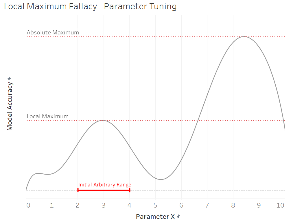
- Fit a model with arbitrary parameter ranges around the defaults.
- If the fitted model picks a boundary value from the parameter range (e.g. range = (1,7) and model picks 7), move the new parameter range to fit 7 inside (e.g. new range = (6, 10)). This would allow me to see if 7 was the best possible value given the original range, or if it was the best possible value regardless of range.
- Repeat this process for every parameter.
Although this may seem like a reasonable approach at first, there are two sources that may introduce error. The first is that I originally picked arbitrary parameter ranges. The issue with doing this is that it’s possible to be optimizing the model to a local maximum instead of the absolute maximum. In other words, steps 2 and 3 may actually be improving the model, but because of the initial placement of parameter ranges, it’s not optimizing the model as much as it could. See the graphic below for a visual representation of this idea.
The second source of error arises because I optimized for one parameter at a time, while thinking I was optimizing them all. To explain this further, I optimized parameter X, given parameter Y and Z stayed the same, while the problem was to optimize them all to get the most optimal model. I then optimized parameter Y, given parameter X and Z stayed the same, and then parameter Z, given X and Y stayed the same. Because the initial parameter values were arbitrarily chosen, we have no confidence, that they will yield the best possible results. This doesn’t necessarily produce the optimal solution to the combination of the parameters, but rather a single parameter, given that all others stay the same.
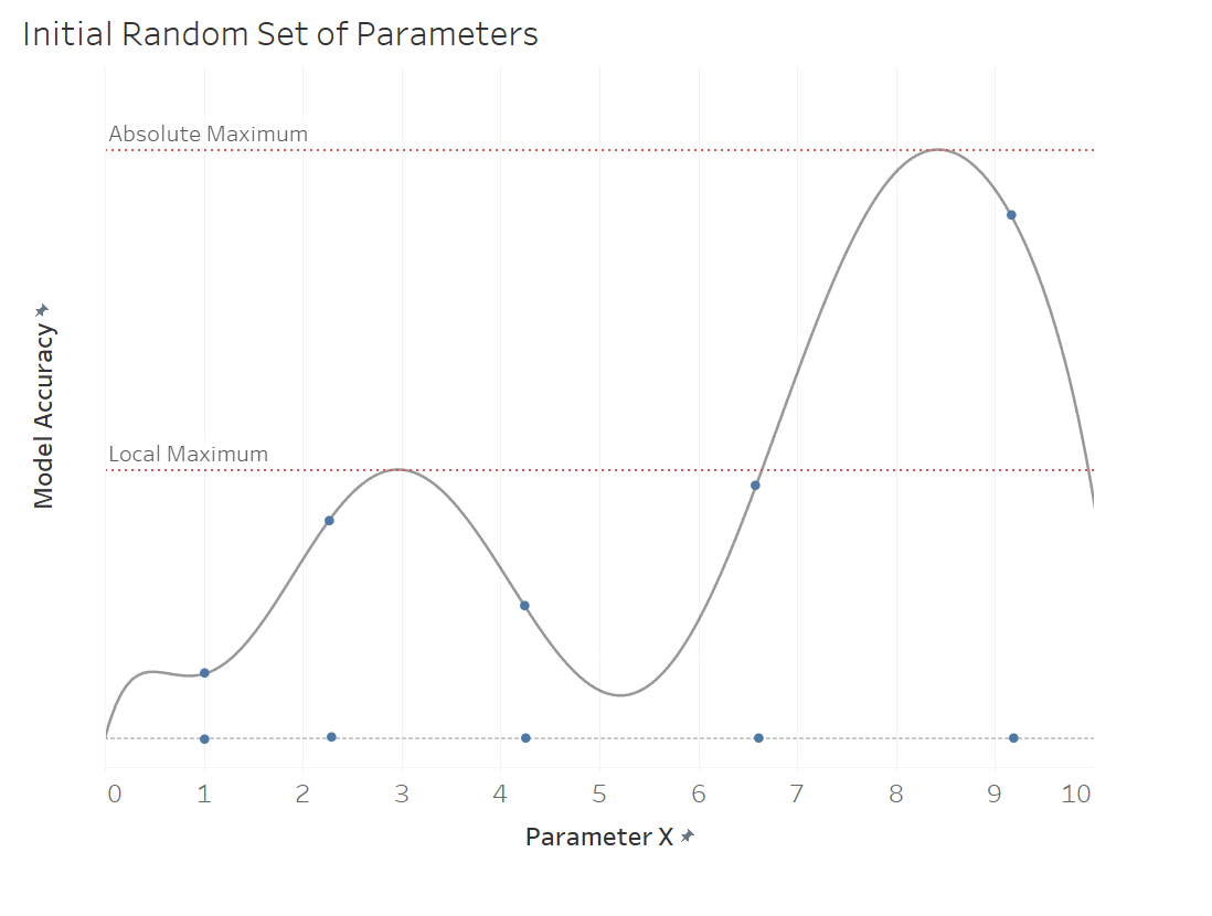
One solution for this is to randomly choose a set amount of parameter combination which, with enough random parameter values, would get rid of the issue of optimizing for a local maximum, as the visualization below shows. We could then use this information to hone in on the parameters that produce the best results, and make more guesses around them. To get rid of the second source of error, we could optimize for all the parameters at the same time. This would be more computationally expensive, but it would guard us against optimizing for one parameter, given that all the others stay the same. To avoid optimizing for a local maximum, we can initially choose several random parameter values and then optimize using the one that yields the highest model accuracy. As mentioned above, in practice, this would be done with a combination of all the parameters of the model, but for the sake of simplicity, it’s illustrated with one parameter. For more information on this topic, please see this in-depth paper on Random Grid Tuning.
Model Ensembling
Perhaps in the second or third iteration of this project, I’d like to learn more about model ensembling and implement it in this project.