Time Series Case Study - Oil Production

Introduction

The goal of this project is to serve as a first glance into the world of time series data analysis. I will analyze US oil production across the years and model the data using a loess model. I will then look at the residuals and decide if a transformation of the data is necessary. Upon performing the transformation, I will compare the two models and pick the one that most closely resembles its data.

Data Overview

I will be using the the US Oil Production dataset, provided by the US Energy Information Administration. The dataset ranges from the year 1920 to the year 2019 and contains information on US oil production. The dataset has two columns: Date, and Prod. Prod is a monthly measurement of the number of barrels of oil that were produced in the US, in thousands of barrels, and Date is the date when the measurement was taken. Below is a snippet of the data.

         Date  Prod
1    Jan-1920  1097
2    Feb-1920  1145
3    Mar-1920  1167
4    Apr-1920  1165
5    May-1920  1181
6    Jun-1920  1222
7    Jul-1920  1218
8    Aug-1920  1255
9    Sep-1920  1251
10   Oct-1920  1277
11   Nov-1920  1287
12   Dec-1920  1257
13   Jan-1921  1230
14   Feb-1921  1269
15   Mar-1921  1326
16   Apr-1921  1341
...

Analysis

The scope of my analysis is to fit a model to the data that can be used for prediction and estimation of US oil production. I will use the LOESS method (local polynomial regression), which works by fitting a linear model across a subset of the data around a particular x and then predicting a y value at that x. It then does the same for all points of the data, with the exception of both endpoints. The resulting curve is plotted by taking all the fitted values from all the regions and connecting them. Span is defined below.

\[span = {2q+1}/{n}\]

Original Data

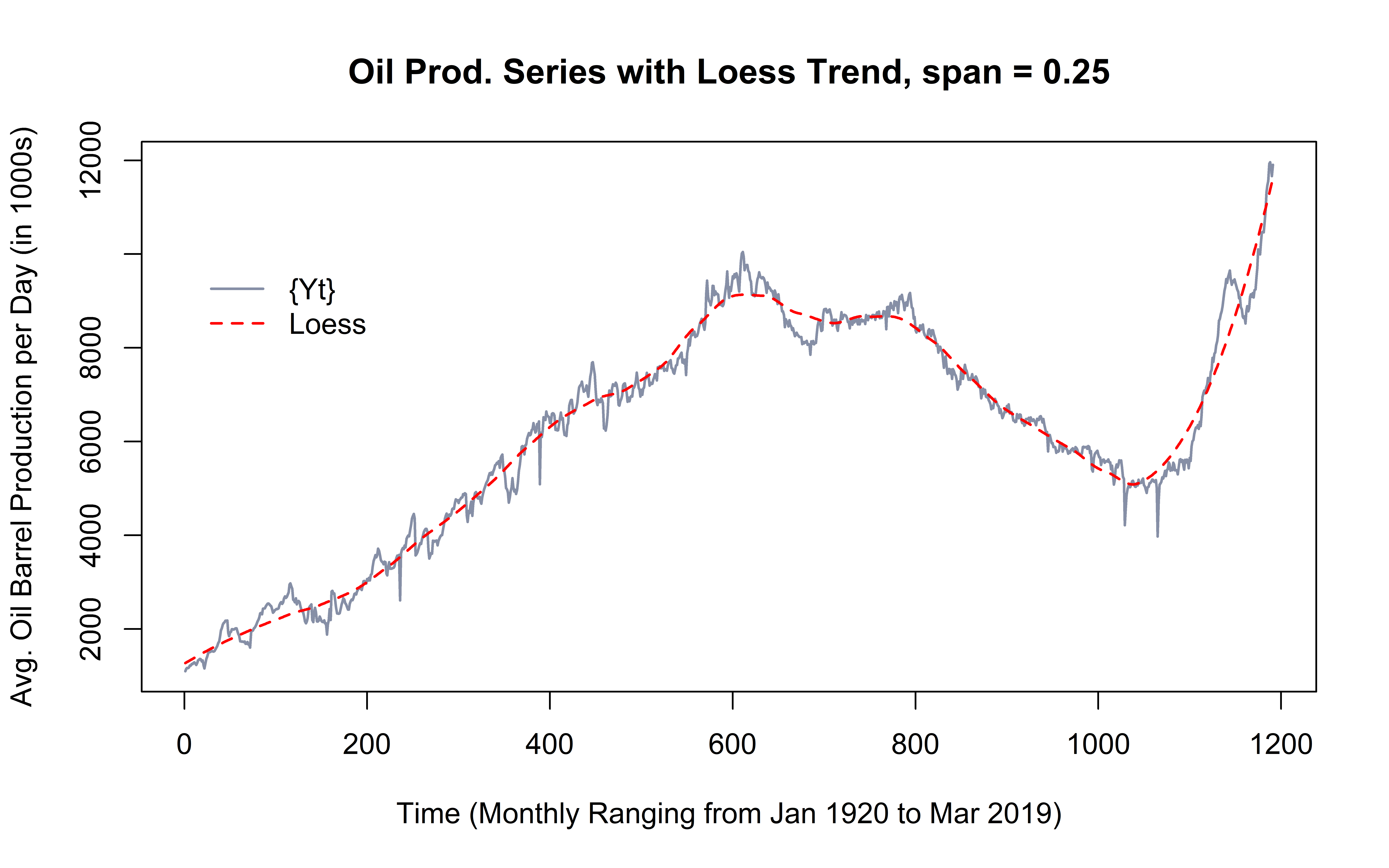
Although there are many ways of picking a span value such as Cross Validation; for the purposes of this report, I will pick the value of 0.25 after visually analyzing the fit of the model with various spans. Below is a line graph of the original data, with a loess model with a span of 0.25 fit in red. The model looks like a good fit as it stays close to the underlying data, while at the same time doesn’t get very jagged. For estimation of values close to the outside the range of the data, this model seems like a good fit.

To get a better idea of whether this model was a good fit, I will analyze the residuals graph (equation shown below) to see if the errors appear to have constant variance and are centered around zero.

\[\hat{X}_{t} = Y_{t}-\hat{m}_{t}\]

From the plot below it looks like the residuals are centered around zero, but there also appears to be a “fanning out” effect for the variance. This leads me to believe that the variance may not be exactly constant, but given the limitations of the scope of this project, this may be the closest estimate. The Corresponding R^2 value (equation shown below) is 0.9822 .

\[R^2 = 1 - {\sum_{t = 1}^N \Big( Y_{t}-\hat{m}_{t} \Big)^2 \over {\sum_{t = 1}^N \Big( Y_{t}-\overline{Y} \Big)^2}}\]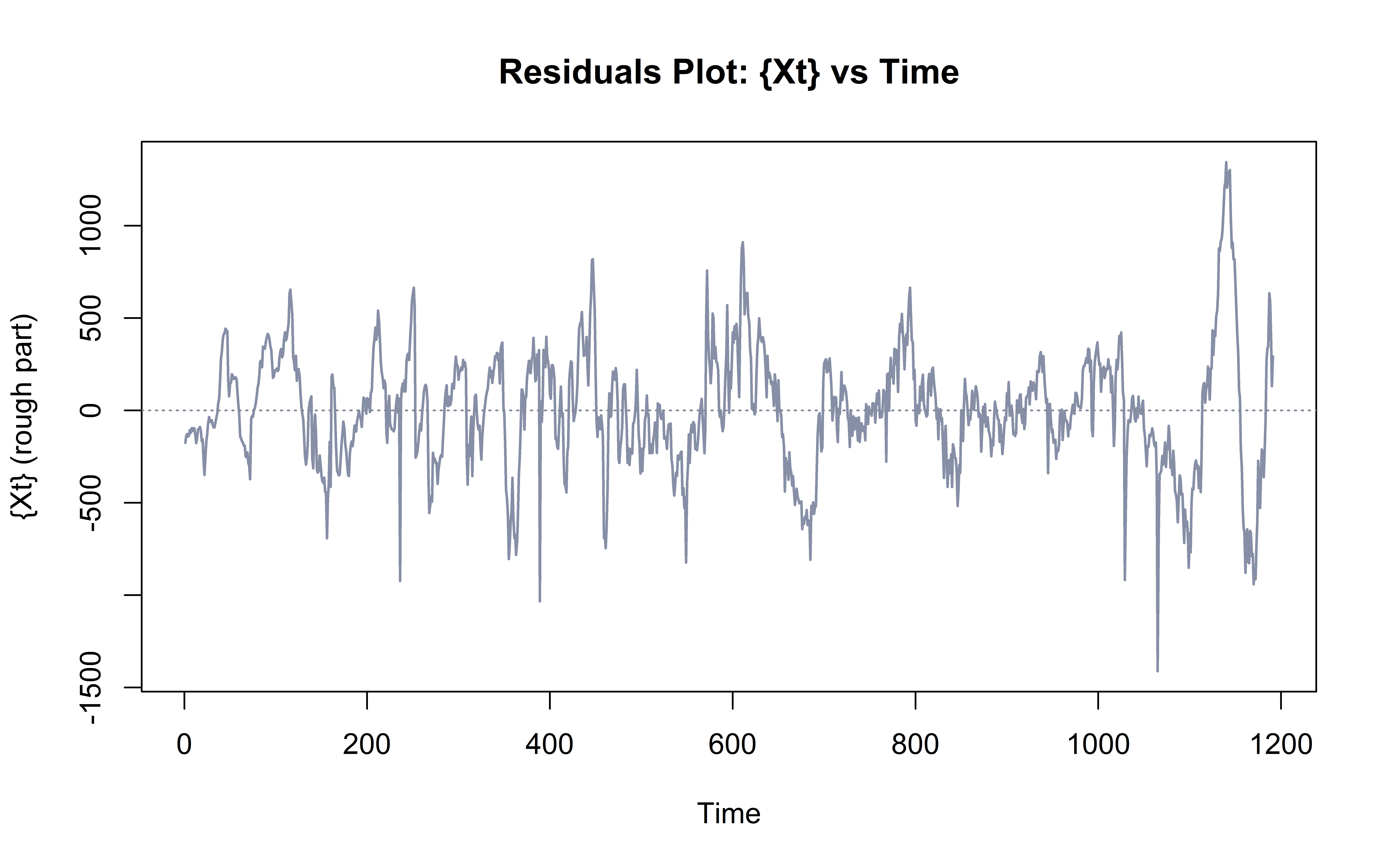

Log of Original Data

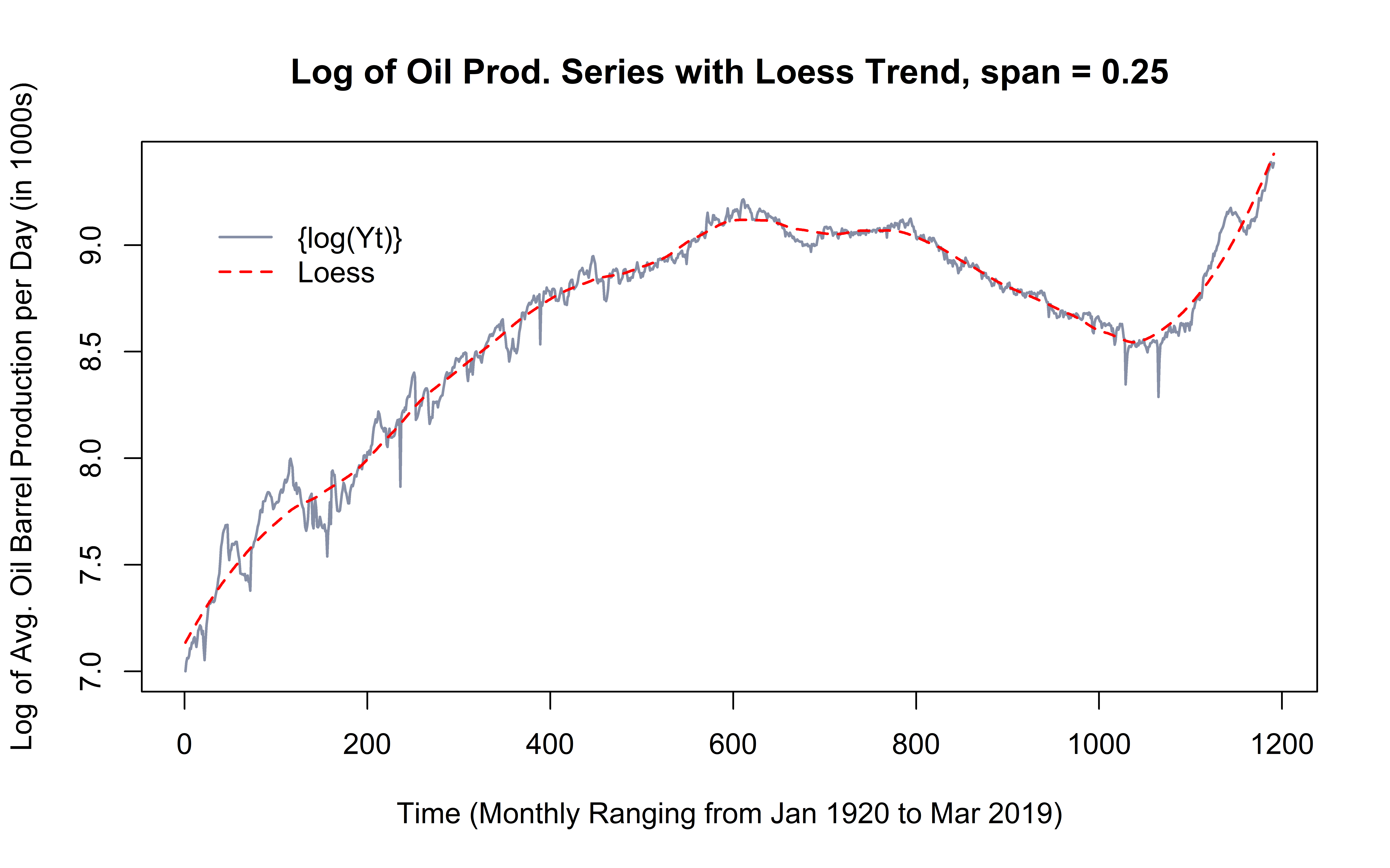
One way to test if it’s possible to get a better fit for the model is by transforming the underlying data and getting a loess curve to the transformed data. As with picking the value for the span, there are many ways to pick a transformation. In this section I will transform the original data by taking its natural log. In the graph below it looks like the model is a closer fit to the log of the original data, which is a promising result for the transformation. But to be sure, I will also analyze the residuals as well as the R^2 value.

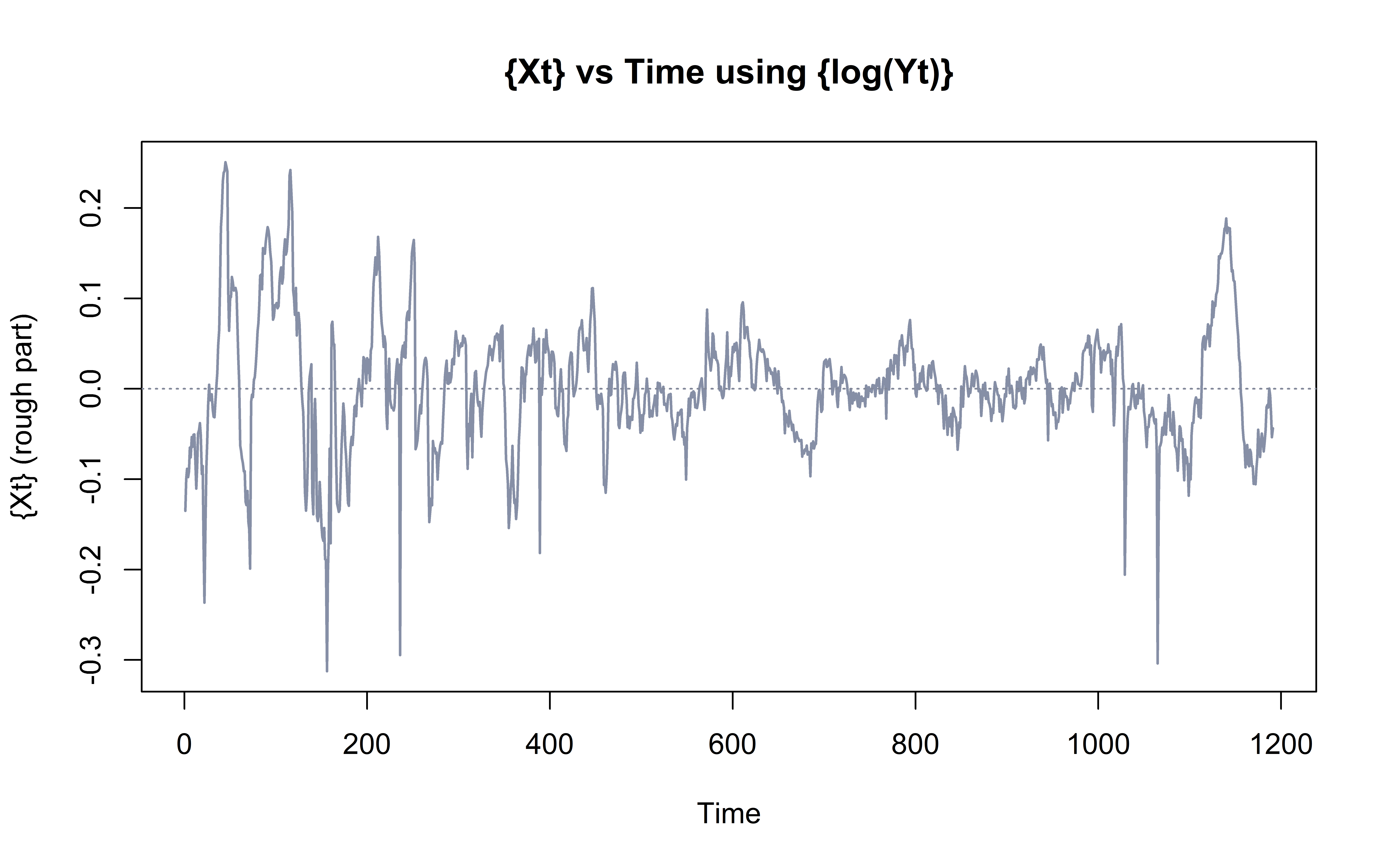
The R^2 value is 0.9828, which is only 0.0006 higher than the R^2 value for the original data. This further confirms that a transformation is not necessary as it doesn’t produce significantly better results.

Results

Even though from the graphs it looked like fitting a loess model over the natural log of the original data was produced a better fit, from the R^2 values, we can see that there is not a significant difference between the two. The R^2 value for the original data is 0.9822, and for the log of the original data it’s 0.9828 . This is not a significant difference, so for the sake of simplicity, it’s best to go with the original data.

Conclusion

In this project I familiarized myself with several key concepts in time series analysis. By looking at Historical Oil Production Data, I first found the trend using a loess model with a span of 0.25. As mentioned above, in future projects, I will use more reliable techniques for selecting the span such as cross validation. Cross validating the data would allow me to test the model on the existing data that I have and not have to wait for future data points to come out. I then transformed the data using a log transformation in order to see if fitting the transformed data yielded better results. Again, I chose this transformation visually for this project, but in the future I will try to select a transformation more objectively, perhaps by analyzing the lambda of a power transformation. All in all, the purpose of this project was fulfilled as I gained a practical application of some fundamental time series concepts.

Analysis and Code

In this section, I include the code that I used to create the visualizations seen in the report.

Loess Trend for Original Data

# Loading the data and changing the column names for ease of use
oil = read.csv("US_oil_prod.csv")
colnames(oil) = c("Date", "Prod")

# Defining the y variable as oil production
y = oil$Prod

# Defining the x (time) variable for every month
time = 1:length(y)

# LOESS model with span = 0.25
loesstrend = loess(y~time, span = 0.25)

# Plotting the data with a thicker line and different color
plot(time, y, type = "l", lty = 1, col = "#868fa6", lwd = 1.5,
  xlab = "Time (Monthly Ranging from Jan 1920 to Mar 2019)",
  ylab = "Avg. Oil Barrel Production per Day (in 1000s)",
  main = "Oil Prod. Series with Loess Trend, span = 0.25")

# Adding the loess model as a red dashed line  
points(time, loesstrend$fit, type = "l", lty = 2, col = "red", lwd = 1.5)

# Specifying the legend location and content
legend(1,10000, c("{Yt}","Loess"),
  lty = c(1,2), col = c("#868fa6", "red"), bty = "n", lwd = 1.5)

Residuals for Original Data

# Plotting the residuals in a similar style to the above graph
plot(time, loesstrend$residuals, type = "l", lty = 1, lwd = 1.5, col ="#868fa6",
  xlab = "Time",
  ylab = "{Xt} (rough part)",
  main = "Residuals Plot: {Xt} vs Time")

# Adding horizontal line at y = 0
abline(h=0, lty = 3, col = "#828899")

Graphs of Log(Orignal Data)

The code to produce the graphs is the same, but log(original data) has to be used now, as defined below.

log_loesstrend = loess(log(y)~time, span = 0.25)